Run this notebook online:![]() or Colab:
or Colab: ![]()
7.4. Networks with Parallel Concatenations (GoogLeNet)
In 2014, [Szegedy et al., 2015] won the ImageNet Challenge, proposing a structure that combined the strengths of the NiN and repeated blocks paradigms. One focus of the paper was to address the question of which sized convolutional kernels are best. After all, previous popular networks employed choices as small as \(1 \times 1\) and as large as \(11 \times 11\). One insight in this paper was that sometimes it can be advantageous to employ a combination of variously-sized kernels. In this section, we will introduce GoogLeNet, presenting a slightly simplified version of the original model—we omit a few ad hoc features that were added to stabilize training but are unnecessary now with better training algorithms available.
7.4.1. Inception Blocks
The basic convolutional block in GoogLeNet is called an Inception block, likely named due to a quote from the movie Inception (“We Need To Go Deeper”), which launched a viral meme.

Fig. 7.4.1 Structure of the Inception block.
As depicted in the figure above, the inception block consists of four parallel paths. The first three paths use convolutional layers with window sizes of \(1\times 1\), \(3\times 3\), and \(5\times 5\) to extract information from different spatial sizes. The middle two paths perform a \(1\times 1\) convolution on the input to reduce the number of input channels, reducing the model’s complexity. The fourth path uses a \(3\times 3\) maximum pooling layer, followed by a \(1\times 1\) convolutional layer to change the number of channels. The four paths all use appropriate padding to give the input and output the same height and width. Finally, the outputs along each path are concatenated along the channel dimension and comprise the block’s output. The commonly-tuned parameters of the Inception block are the number of output channels per layer.
%load ../utils/djl-imports
%load ../utils/plot-utils
%load ../utils/Training.java
%load ../utils/Accumulator.java
import ai.djl.basicdataset.cv.classification.*;
import org.apache.commons.lang3.ArrayUtils;
import java.util.stream.*;
// c1 - c4 are the number of output channels for each layer in the path
public ParallelBlock inceptionBlock(int c1, int[] c2, int[] c3, int c4) {

    // Path 1 is a single 1 x 1 convolutional layer
    SequentialBlock p1 = new SequentialBlock().add(
            Conv2d.builder()
                    .setFilters(c1)
                    .setKernelShape(new Shape(1, 1))
                    .build())
            .add(Activation::relu);

    // Path 2 is a 1 x 1 convolutional layer followed by a 3 x 3
    // convolutional layer
    SequentialBlock p2 = new SequentialBlock().add(
            Conv2d.builder()
                    .setFilters(c2[0])
                    .setKernelShape(new Shape(1, 1))
                    .build())
            .add(Activation::relu)
            .add(
                    Conv2d.builder()
                            .setFilters(c2[1])
                            .setKernelShape(new Shape(3, 3))
                            .optPadding(new Shape(1, 1))
                            .build())
            .add(Activation::relu);

    // Path 3 is a 1 x 1 convolutional layer followed by a 5 x 5
    // convolutional layer
    SequentialBlock p3 = new SequentialBlock().add(
            Conv2d.builder()
                    .setFilters(c3[0])
                    .setKernelShape(new Shape(1, 1))
                    .build())
            .add(Activation::relu)
            .add(
                    Conv2d.builder()
                            .setFilters(c3[1])
                            .setKernelShape(new Shape(5, 5))
                            .optPadding(new Shape(2, 2))
                            .build())
            .add(Activation::relu);

    // Path 4 is a 3 x 3 maximum pooling layer followed by a 1 x 1
    // convolutional layer
    SequentialBlock p4 = new SequentialBlock()
            .add(Pool.maxPool2dBlock(new Shape(3, 3), new Shape(1, 1), new Shape(1, 1)))
            .add(Conv2d.builder()
                    .setFilters(c4)
                    .setKernelShape(new Shape(1, 1))
                    .build())
            .add(Activation::relu);

    // Concatenate the outputs on the channel dimension
    return new ParallelBlock(
                        list -> {
                            List<NDArray> concatenatedList = list
                                    .stream()
                                    .map(NDList::head)
                                    .collect(Collectors.toList());

                            return new NDList(NDArrays.concat(new NDList(concatenatedList), 1));
                        }, Arrays.asList(p1, p2, p3, p4));
}
To gain some intuition for why this network works so well, consider the combination of the filters. They explore the image in varying ranges. This means that details at different extents can be recognized efficiently by different filters. At the same time, we can allocate different amounts of parameters for different ranges (e.g., more for short range but not ignore the long range entirely).
7.4.2. GoogLeNet Model
As shown in Fig. 7.4.2, GoogLeNet uses a stack of a total of 9 inception blocks and global average pooling to generate its estimates. Maximum pooling between inception blocks reduced the dimensionality. The first part is identical to AlexNet and LeNet, the stack of blocks is inherited from VGG and the global average pooling avoids a stack of fully-connected layers at the end. The architecture is depicted below.

Fig. 7.4.2 Full GoogLeNet Model
We can now implement GoogLeNet piece by piece. The first component uses a 64-channel \(7\times 7\) convolutional layer.
SequentialBlock block1 = new SequentialBlock();
block1
    .add(Conv2d.builder()
                .setKernelShape(new Shape(7, 7))
                .optPadding(new Shape(3, 3))
                .optStride(new Shape(2, 2))
                .setFilters(64)
                .build())
    .add(Activation::relu)
    .add(Pool.maxPool2dBlock(new Shape(3, 3), new Shape(2, 2), new Shape(1, 1)));
SequentialBlock {
    Conv2d
    LambdaBlock
    maxPool2d
}
The second component uses two convolutional layers: first, a 64-channel \(1\times 1\) convolutional layer, then a \(3\times 3\) convolutional layer that triples the number of channels. This corresponds to the second path in the Inception block.
SequentialBlock block2 = new SequentialBlock();
block2
    .add(Conv2d.builder()
            .setFilters(64)
            .setKernelShape(new Shape(1, 1))
            .build())
    .add(Activation::relu)
    .add(Conv2d.builder()
            .setFilters(192)
            .setKernelShape(new Shape(3, 3))
            .optPadding(new Shape(1, 1))
            .build())
    .add(Activation::relu)
    .add(Pool.maxPool2dBlock(new Shape(3, 3), new Shape(2, 2), new Shape(1, 1)));
SequentialBlock {
    Conv2d
    LambdaBlock
    Conv2d
    LambdaBlock
    maxPool2d
}
The third component connects two complete Inception blocks in series. The number of output channels of the first Inception block is \(64+128+32+32=256\), and the ratio to the output channels of the four paths is \(64:128:32:32=2:4:1:1\). The second and third paths first reduce the number of input channels to \(96/192=1/2\) and \(16/192=1/12\), respectively, and then connect the second convolutional layer. The number of output channels of the second Inception block is increased to \(128+192+96+64=480\), and the ratio to the number of output channels per path is \(128:192:96:64 = 4:6:3:2\). The second and third paths first reduce the number of input channels to \(128/256=1/2\) and \(32/256=1/8\), respectively.
SequentialBlock block3 = new SequentialBlock();
block3
        .add(inceptionBlock(64, new int[]{96, 128}, new int[]{16, 32}, 32))
        .add(inceptionBlock(128, new int[]{128, 192}, new int[]{32, 96}, 64))
        .add(Pool.maxPool2dBlock(new Shape(3, 3), new Shape(2, 2), new Shape(1, 1)));
SequentialBlock {
    ParallelBlock {
            SequentialBlock {
                    Conv2d
                    LambdaBlock
            }
            SequentialBlock {
                    Conv2d
                    LambdaBlock
                    Conv2d
                    LambdaBlock
            }
            SequentialBlock {
                    Conv2d
                    LambdaBlock
                    Conv2d
                    LambdaBlock
            }
            SequentialBlock {
                    maxPool2d
                    Conv2d
                    LambdaBlock
            }
    }
    maxPool2d
}
The fourth block is more complicated. It connects five Inception blocks in series, and they have \(192+208+48+64=512\), \(160+224+64+64=512\), \(128+256+64+64=512\), \(112+288+64+64=528\), and \(256+320+128+128=832\) output channels, respectively. The number of channels assigned to these paths is similar to that in the third module: the second path with the \(3\times 3\) convolutional layer outputs the largest number of channels, followed by the first path with only the \(1\times 1\) convolutional layer, the third path with the \(5\times 5\) convolutional layer, and the fourth path with the \(3\times 3\) maximum pooling layer. The second and third paths will first reduce the number of channels according the ratio. These ratios are slightly different in different Inception blocks.
SequentialBlock block4 = new SequentialBlock();
block4
        .add(inceptionBlock(192, new int[]{96, 208}, new int[]{16, 48}, 64))
        .add(inceptionBlock(160, new int[]{112, 224}, new int[]{24, 64}, 64))
        .add(inceptionBlock(128, new int[]{128, 256}, new int[]{24, 64}, 64))
        .add(inceptionBlock(112, new int[]{144, 288}, new int[]{32, 64}, 64))
        .add(inceptionBlock(256, new int[]{160, 320}, new int[]{32, 128}, 128))
        .add(Pool.maxPool2dBlock(new Shape(3, 3), new Shape(2, 2), new Shape(1, 1)));
SequentialBlock {
    ParallelBlock {
            SequentialBlock {
                    Conv2d
                    LambdaBlock
            }
            SequentialBlock {
                    Conv2d
                    LambdaBlock
                    Conv2d
                    LambdaBlock
            }
            SequentialBlock {
                    Conv2d
                    LambdaBlock
                    Conv2d
                    LambdaBlock
            }
            SequentialBlock {
                    maxPool2d
                    Conv2d
                    LambdaBlock
            }
    }
    ParallelBlock {
            SequentialBlock {
                    Conv2d
                    LambdaBlock
            }
            SequentialBlock {
                    Conv2d
                    LambdaBlock
                    Conv2d
                    LambdaBlock
            }
            SequentialBlock {
                    Conv2d
                    LambdaBlock
                    Conv2d
                    LambdaBlock
            }
            SequentialBlock {
                    maxPool2d
                    Conv2d
                    LambdaBlock
            }
    }
    maxPool2d
}
The fifth block has two Inception blocks with \(256+320+128+128=832\) and \(384+384+128+128=1024\) output channels. The number of channels assigned to each path is the same as that in the third and fourth modules, but differs in specific values. It should be noted that the fifth block is followed by the output layer. This block uses the global average pooling layer to change the height and width of each channel to 1, just as in NiN. Finally, we turn the output into a two-dimensional array followed by a fully-connected layer whose number of outputs is the number of label classes.
SequentialBlock block5 = new SequentialBlock();
block5
        .add(inceptionBlock(256, new int[]{160, 320}, new int[]{32, 128}, 128))
        .add(inceptionBlock(384, new int[]{192, 384}, new int[]{48, 128}, 128))
        .add(Pool.globalAvgPool2dBlock());

SequentialBlock block = new SequentialBlock();
block = block.addAll(block1, block2, block3, block4, block5, Linear.builder().setUnits(10).build());
The GoogLeNet model is computationally complex, so it is not as easy to modify the number of channels as in VGG. To have a reasonable training time on Fashion-MNIST, we reduce the input height and width from 224 to 96. This simplifies the computation. The changes in the shape of the output between the various modules is demonstrated below.
NDManager manager = NDManager.newBaseManager();
float lr = 0.1f;
Model model = Model.newInstance("cnn");
model.setBlock(block);

Loss loss = Loss.softmaxCrossEntropyLoss();

Tracker lrt = Tracker.fixed(lr);
Optimizer sgd = Optimizer.sgd().setLearningRateTracker(lrt).build();

DefaultTrainingConfig config = new DefaultTrainingConfig(loss).optOptimizer(sgd) // Optimizer (loss function)
        .optDevices(Engine.getInstance().getDevices(1)) // single GPU
        .addEvaluator(new Accuracy()) // Model Accuracy
        .addTrainingListeners(TrainingListener.Defaults.logging()); // Logging

Trainer trainer = model.newTrainer(config);

NDArray X = manager.randomUniform(0f, 1.0f, new Shape(1, 1, 96, 96));
trainer.initialize(X.getShape());
Shape currentShape = X.getShape();

for (int i = 0; i < block.getChildren().size(); i++) {
    Shape[] newShape = block.getChildren().get(i).getValue().getOutputShapes(new Shape[]{currentShape});
    currentShape = newShape[0];
    System.out.println(block.getChildren().get(i).getKey()+ i + " layer output : " + currentShape);
}
INFO Training on: 1 GPUs.
INFO Load MXNet Engine Version 1.9.0 in 0.055 ms.
01SequentialBlock0 layer output : (1, 64, 24, 24)
02SequentialBlock1 layer output : (1, 192, 12, 12)
03SequentialBlock2 layer output : (1, 480, 6, 6)
04SequentialBlock3 layer output : (1, 832, 3, 3)
05SequentialBlock4 layer output : (1, 1024)
06Linear5 layer output : (1, 10)
7.4.3. Data Acquisition and Training
As before, we train our model using the Fashion-MNIST dataset. We transform it to \(96 \times 96\) pixel resolution before invoking the training procedure.
int batchSize = 128;
int numEpochs = Integer.getInteger("MAX_EPOCH", 10);

double[] trainLoss;
double[] testAccuracy;
double[] epochCount;
double[] trainAccuracy;

epochCount = new double[numEpochs];

for (int i = 0; i < epochCount.length; i++) {
    epochCount[i] = (i + 1);
}

FashionMnist trainIter = FashionMnist.builder()
        .addTransform(new Resize(96))
        .addTransform(new ToTensor())
        .optUsage(Dataset.Usage.TRAIN)
        .setSampling(batchSize, true)
        .optLimit(Long.getLong("DATASET_LIMIT", Long.MAX_VALUE))
        .build();

FashionMnist testIter = FashionMnist.builder()
        .addTransform(new Resize(96))
        .addTransform(new ToTensor())
        .optUsage(Dataset.Usage.TEST)
        .setSampling(batchSize, true)
        .optLimit(Long.getLong("DATASET_LIMIT", Long.MAX_VALUE))
        .build();

trainIter.prepare();
testIter.prepare();
Map<String, double[]> evaluatorMetrics = new HashMap<>();
double avgTrainTimePerEpoch = Training.trainingChapter6(trainIter, testIter, numEpochs, trainer, evaluatorMetrics);
Training:    100% |████████████████████████████████████████| Accuracy: 0.20, SoftmaxCrossEntropyLoss: 2.16
Validating:  100% |████████████████████████████████████████|
INFO Epoch 1 finished.
INFO Train: Accuracy: 0.20, SoftmaxCrossEntropyLoss: 2.15
INFO Validate: Accuracy: 0.39, SoftmaxCrossEntropyLoss: 1.70
Training:    100% |████████████████████████████████████████| Accuracy: 0.64, SoftmaxCrossEntropyLoss: 0.93
Validating:  100% |████████████████████████████████████████|
INFO Epoch 2 finished.
INFO Train: Accuracy: 0.64, SoftmaxCrossEntropyLoss: 0.93
INFO Validate: Accuracy: 0.71, SoftmaxCrossEntropyLoss: 0.75
Training:    100% |████████████████████████████████████████| Accuracy: 0.82, SoftmaxCrossEntropyLoss: 0.49
Validating:  100% |████████████████████████████████████████|
INFO Epoch 3 finished.
INFO Train: Accuracy: 0.82, SoftmaxCrossEntropyLoss: 0.49
INFO Validate: Accuracy: 0.83, SoftmaxCrossEntropyLoss: 0.45
Training:    100% |████████████████████████████████████████| Accuracy: 0.86, SoftmaxCrossEntropyLoss: 0.37
Validating:  100% |████████████████████████████████████████|
INFO Epoch 4 finished.
INFO Train: Accuracy: 0.86, SoftmaxCrossEntropyLoss: 0.37
INFO Validate: Accuracy: 0.87, SoftmaxCrossEntropyLoss: 0.34
Training:    100% |████████████████████████████████████████| Accuracy: 0.88, SoftmaxCrossEntropyLoss: 0.32
Validating:  100% |████████████████████████████████████████|
INFO Epoch 5 finished.
INFO Train: Accuracy: 0.88, SoftmaxCrossEntropyLoss: 0.32
INFO Validate: Accuracy: 0.88, SoftmaxCrossEntropyLoss: 0.34
Training:    100% |████████████████████████████████████████| Accuracy: 0.89, SoftmaxCrossEntropyLoss: 0.28
Validating:  100% |████████████████████████████████████████|
INFO Epoch 6 finished.
INFO Train: Accuracy: 0.89, SoftmaxCrossEntropyLoss: 0.28
INFO Validate: Accuracy: 0.89, SoftmaxCrossEntropyLoss: 0.30
Training:    100% |████████████████████████████████████████| Accuracy: 0.90, SoftmaxCrossEntropyLoss: 0.26
Validating:  100% |████████████████████████████████████████|
INFO Epoch 7 finished.
INFO Train: Accuracy: 0.90, SoftmaxCrossEntropyLoss: 0.26
INFO Validate: Accuracy: 0.90, SoftmaxCrossEntropyLoss: 0.27
Training:    100% |████████████████████████████████████████| Accuracy: 0.49, SoftmaxCrossEntropyLoss: 1.35
Validating:  100% |████████████████████████████████████████|
INFO Epoch 8 finished.
INFO Train: Accuracy: 0.49, SoftmaxCrossEntropyLoss: 1.35
INFO Validate: Accuracy: 0.77, SoftmaxCrossEntropyLoss: 0.63
Training:    100% |████████████████████████████████████████| Accuracy: 0.82, SoftmaxCrossEntropyLoss: 0.48
Validating:  100% |████████████████████████████████████████|
INFO Epoch 9 finished.
INFO Train: Accuracy: 0.82, SoftmaxCrossEntropyLoss: 0.48
INFO Validate: Accuracy: 0.84, SoftmaxCrossEntropyLoss: 0.42
Training:    100% |████████████████████████████████████████| Accuracy: 0.86, SoftmaxCrossEntropyLoss: 0.37
Validating:  100% |████████████████████████████████████████|
INFO Epoch 10 finished.
INFO Train: Accuracy: 0.86, SoftmaxCrossEntropyLoss: 0.37
INFO Validate: Accuracy: 0.81, SoftmaxCrossEntropyLoss: 0.54
trainLoss = evaluatorMetrics.get("train_epoch_SoftmaxCrossEntropyLoss");
trainAccuracy = evaluatorMetrics.get("train_epoch_Accuracy");
testAccuracy = evaluatorMetrics.get("validate_epoch_Accuracy");

System.out.printf("loss %.3f,", trainLoss[numEpochs - 1]);
System.out.printf(" train acc %.3f,", trainAccuracy[numEpochs - 1]);
System.out.printf(" test acc %.3f\n", testAccuracy[numEpochs - 1]);
System.out.printf("%.1f examples/sec", trainIter.size() / (avgTrainTimePerEpoch / Math.pow(10, 9)));
System.out.println();
loss 0.368, train acc 0.860, test acc 0.810
1684.3 examples/sec
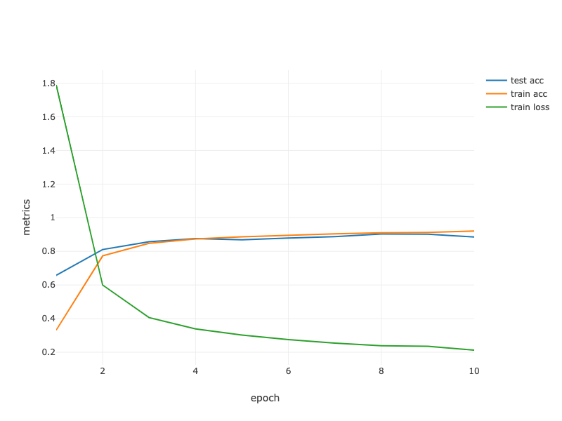
Fig. 7.4.3 Contour Gradient Descent.
String[] lossLabel = new String[trainLoss.length + testAccuracy.length + trainAccuracy.length];

Arrays.fill(lossLabel, 0, trainLoss.length, "train loss");
Arrays.fill(lossLabel, trainAccuracy.length, trainLoss.length + trainAccuracy.length, "train acc");
Arrays.fill(lossLabel, trainLoss.length + trainAccuracy.length,
                trainLoss.length + testAccuracy.length + trainAccuracy.length, "test acc");

Table data = Table.create("Data").addColumns(
    DoubleColumn.create("epoch", ArrayUtils.addAll(epochCount, ArrayUtils.addAll(epochCount, epochCount))),
    DoubleColumn.create("metrics", ArrayUtils.addAll(trainLoss, ArrayUtils.addAll(trainAccuracy, testAccuracy))),
    StringColumn.create("lossLabel", lossLabel)
);

render(LinePlot.create("", data, "epoch", "metrics", "lossLabel"),"text/html");
7.4.4. Summary
The Inception block is equivalent to a subnetwork with four paths. It extracts information in parallel through convolutional layers of different window shapes and maximum pooling layers. \(1 \times 1\) convolutions reduce channel dimensionality on a per-pixel level. Max-pooling reduces the resolution.
GoogLeNet connects multiple well-designed Inception blocks with other layers in series. The ratio of the number of channels assigned in the Inception block is obtained through a large number of experiments on the ImageNet dataset.
GoogLeNet, as well as its succeeding versions, was one of the most efficient models on ImageNet, providing similar test accuracy with lower computational complexity.
7.4.5. Exercises
There are several iterations of GoogLeNet. Try to implement and run them. Some of them include the following:
Add a batch normalization layer [Ioffe & Szegedy, 2015], as described later in Section 7.5.
Make adjustments to the Inception block [Szegedy et al., 2016].
Use “label smoothing” for model regularization [Szegedy et al., 2016].
Include it in the residual connection [Szegedy et al., 2017], as described later in Section 7.6.
What is the minimum image size for GoogLeNet to work?
Compare the model parameter sizes of AlexNet, VGG, and NiN with GoogLeNet. How do the latter two network architectures significantly reduce the model parameter size?
Why do we need a large range convolution initially?