Run this notebook online:![]() or Colab:
or Colab: ![]()
3.6. softmax回归的从零开始实现
就像我们从零开始实现线性回归一样,我们认为softmax回归也是重要的基础,因此你应该知道实现softmax的细节。我们使用刚刚在 Section 3.5 中引入的Fashion-MNIST数据集,并设置数据迭代器的批量大小为256。
%load ../utils/djl-imports
%load ../utils/plot-utils.ipynb
%load ../utils/Training.java
%load ../utils/FashionMnistUtils.java
%load ../utils/ImageUtils.java

import ai.djl.basicdataset.cv.classification.*;
int batchSize = 256;
boolean randomShuffle = true;

// get training and validation dataset
FashionMnist trainingSet = FashionMnist.builder()
        .optUsage(Dataset.Usage.TRAIN)
        .setSampling(batchSize, randomShuffle)
        .optLimit(Long.getLong("DATASET_LIMIT", Long.MAX_VALUE))
        .build();

FashionMnist validationSet = FashionMnist.builder()
        .optUsage(Dataset.Usage.TEST)
        .setSampling(batchSize, false)
        .optLimit(Long.getLong("DATASET_LIMIT", Long.MAX_VALUE))
        .build();
3.6.1. 初始化模型参数
和之前线性回归的例子一样,这里的每个样本都将用固定长度的向量表示。原始数据集中的每个样本都是 \(28 \times 28\) 的图像。在本节中,我们将展平每个图像,把它们看作长度为784的向量。在后面的章节中,将讨论能够利用图像空间结构的更为复杂的策略,但现在我们暂时只把每个像素位置看作一个特征。
回想一下,在softmax回归中,我们的输出与类别一样多。因为我们的数据集有10个类别,所以网络输出维度为
10。因此,权重将构成一个 \(784 \times 10\) 的矩阵,偏置将构成一个
\(1 \times 10\)
的行向量。与线性回归一样,我们将使用正态分布初始化我们的权重
W,偏置初始化为0。
int numInputs = 784;
int numOutputs = 10;

NDManager manager = NDManager.newBaseManager();
NDArray W = manager.randomNormal(0, 0.01f, new Shape(numInputs, numOutputs), DataType.FLOAT32);
NDArray b = manager.zeros(new Shape(numOutputs), DataType.FLOAT32);
NDList params = new NDList(W, b);
3.6.2. 定义softmax操作
在实现softmax回归模型之前,让我们简要地回顾一下sum()运算符如何沿着NDArray中的特定维度工作,如
Section 2.3.6 和
Section 2.3.6.1
所述。给定一个矩阵X,我们可以对所有元素求和(默认情况下),也可以只求同一个轴上的元素,即同一列new int[]{0}或同一行new int[]{0, 1}。如果
X 是一个形状为 (2, 3)
的NDArray,我们对列进行求和,则结果将是一个具有形状 (3,)
的向量。当调用sum运算符时,我们可以指定保持在原始 NDArray
的轴数,而不折叠求和的维度。这将产生一个具有形状 (1, 3) 的二维
NDArray 。
NDArray X = manager.create(new int[][]{{1, 2, 3}, {4, 5, 6}});
System.out.println(X.sum(new int[]{0}, true));
System.out.println(X.sum(new int[]{1}, true));
System.out.println(X.sum(new int[]{0, 1}, true));
ND: (1, 3) gpu(0) int32
[[ 5,  7,  9],
]

ND: (2, 1) gpu(0) int32
[[ 6],
 [15],
]

ND: (1, 1) gpu(0) int32
[[21],
]
我们现在已经准备好实现softmax操作了。回想一下,softmax 由三个步骤组成:
对每个项求幂(使用
exp())。对每一行求和(小批量中每个样本是一行),得到每个样本的归一化常数。
将每一行除以其归一化常数,确保结果的和为1。
在查看代码之前,让我们回顾一下这个表达式:
分母或归一化常数,有时也称为配分函数(其对数称为对数-配分函数)。该名称的起源来自 统计物理学中一个模拟粒子群分布的方程。
public NDArray softmax(NDArray X) {
    NDArray Xexp = X.exp();
    NDArray partition = Xexp.sum(new int[]{1}, true);
    return Xexp.div(partition); // 这里应用了广播机制
}
正如你所看到的,对于任何随机输入,我们将每个元素变成一个非负数。此外,依据概率原理,每行总和为1。注意,虽然这在数学上看起来是正确的,但我们在代码实现中有点草率。矩阵中的非常大或非常小的元素可能造成数值上溢或下溢,但我们没有采取措施来防止这点。
NDArray X = manager.randomNormal(new Shape(2, 5));
NDArray Xprob = softmax(X);
System.out.println(Xprob);
System.out.println(Xprob.sum(new int[]{1}));
ND: (2, 5) gpu(0) float32
[[0.1406, 0.117 , 0.5391, 0.0491, 0.1541],
 [0.204 , 0.0605, 0.0759, 0.5691, 0.0905],
]

ND: (2) gpu(0) float32
[1.    , 1.    ]
3.6.3. 定义模型
现在我们已经定义了softmax操作,我们可以实现softmax回归模型。下面的代码定义了输入如何通过网络映射到输出。注意,在将数据传递到我们的模型之前,我们使用
reshape() 函数将每张原始图像展平为向量。
// We need to wrap `net()` in a class so that we can reference the method
// and pass it as a parameter to a function or save it in a variable
public class Net {
    public static NDArray net(NDArray X) {
        NDArray currentW = params.get(0);
        NDArray currentB = params.get(1);
        return softmax(X.reshape(new Shape(-1, numInputs)).dot(currentW).add(currentB));
    }
}
3.6.4. 定义损失函数
接下来,我们需要实现 Section 3.4 中引入的交叉熵损失函数。这可能是深度学习中最常见的损失函数,因为目前分类问题的数量远远超过回归问题。
回顾一下,交叉熵采用真实标签的预测概率的负对数似然。我们不需要使用Java的for循环迭代预测(这往往是低效的)。
我们可以使用 NDIndex 表达式选择 NDArray
索引的元素,下面,我们创建一个数据yHat,其中包含2个样本在3个类别的预测概率,我们知道在第一个样本中,第一类是正确的预测,而在第二个样本中,第三类是正确的预测。我们可以使用
“:, {}” 表达式选择正确的预测。 NDArray: {0, 2} 作为 yHat
中概率的索引,表示选择第一个样本中第 0 列和第二个样本中 2 列。
注意:创建 NDIndex 时使用的 NDArray 的数据类型必须是 int 或
long。你需要使用 toType() 函数将非整形 NDArray 转成
DataType.INT32 或 DataType.INT64。
NDArray yHat = manager.create(new float[][]{{0.1f, 0.3f, 0.6f}, {0.3f, 0.2f, 0.5f}});
yHat.get(new NDIndex(":, {}", manager.create(new int[]{0, 2})));
ND: (2, 2) gpu(0) float32
[[0.1, 0.6],
 [0.3, 0.5],
]
现在我们只需一行代码就可以实现交叉熵损失函数。
// Cross Entropy only cares about the target class's probability
// Get the column index for each row
public class LossFunction {
    public static NDArray crossEntropy(NDArray yHat, NDArray y) {
        // Here, y is not guranteed to be of datatype int or long
        // and in our case we know its a float32.
        // We must first convert it to int or long(here we choose int)
        // before we can use it with NDIndex to "pick" indices.
        // It also takes in a boolean for returning a copy of the existing NDArray
        // but we don't want that so we pass in `false`.
        NDIndex pickIndex = new NDIndex()
                 .addAllDim(Math.floorMod(-1, yHat.getShape().dimension()))
                 .addPickDim(y);
        return yHat.get(pickIndex).log().neg();
    }
}
3.6.5. 分类准确率
给定预测概率分布 yHat,当我们必须输出硬预测(hard
prediction)时,我们通常选择预测概率最高的类。许多应用都要求我们做出选择。如Gmail必须将电子邮件分为“Primary(主要)”、“Social(社交)”、“Updates(更新)”或“Forums(论坛)”。它可能在内部估计概率,但最终它必须在类中选择一个。
当预测与标签分类 y
一致时,它们是正确的。分类准确率即正确预测数量与总预测数量之比。虽然直接优化准确率可能很困难(因为准确率的计算不可导),但准确率通常是我们最关心的性能衡量标准,我们在训练分类器时几乎总是会报告它。
为了计算准确率,我们执行以下操作。首先,如果 yHat
是矩阵,那么假定第二个维度存储每个类的预测分数。我们使用
yHat.argMax()
获得每行中最大元素的索引来获得预测类别。然后我们将预测类别与真实 y
元素进行比较。由于 eq() 函数要求数据类型也一致,因此我们将 yHat
的数据类型转换为与 y 相同的数据类型。结果是一个包含 0(错)和
1(对)的 NDArray。进行求和会得到正确预测的数量。
// Saved in the utils for later use
public float accuracy(NDArray yHat, NDArray y) {
    // Check size of 1st dimension greater than 1
    // to see if we have multiple samples
    if (yHat.getShape().size(1) > 1) {
        // Argmax gets index of maximum args for given axis 1
        // Convert yHat to same dataType as y (int32)
        // Sum up number of true entries
        return yHat.argMax(1).toType(DataType.INT32, false).eq(y.toType(DataType.INT32, false))
            .sum().toType(DataType.FLOAT32, false).getFloat();
    }
    return yHat.toType(DataType.INT32, false).eq(y.toType(DataType.INT32, false))
        .sum().toType(DataType.FLOAT32, false).getFloat();
}
我们将继续使用之前定义的变量 yHat 和 y
分别作为预测的概率分布和标签。我们可以看到,第一个样本的预测类别是2(该行的最大元素为0.6,索引为2),这与实际标签0不一致。第二个样本的预测类别是2(该行的最大元素为0.5,索引为
2),这与实际标签2一致。因此,这两个样本的分类准确率率为0.5。
NDArray y = manager.create(new int[]{0,2});
accuracy(yHat, y) / y.size();
0.5
同样,对于任意数据迭代器 dataIterator
可访问的数据集,我们可以评估在任意模型 net 的准确率。
import java.util.function.UnaryOperator;
import java.util.function.BinaryOperator;
// Saved in the utils for future use
public float evaluateAccuracy(UnaryOperator<NDArray> net, Iterable<Batch> dataIterator) {
    Accumulator metric = new Accumulator(2);  // numCorrectedExamples, numExamples
    for (Batch batch : dataIterator) {
        NDArray X = batch.getData().head();
        NDArray y = batch.getLabels().head();
        metric.add(new float[]{accuracy(net.apply(X), y), (float)y.size()});
        batch.close();
    }
    return metric.get(0) / metric.get(1);
}
这里 Accumulator 是一个实用程序类,用于对多个变量进行累加。
// Saved in utils for future use
/* Sum a list of numbers over time */
public class Accumulator {
    float[] data;

    public Accumulator(int n) {
        data = new float[n];
    }

    /* Adds a set of numbers to the array */
    public void add(float[] args) {
        for (int i = 0; i < args.length; i++) {
            data[i] += args[i];
        }
    }

    /* Resets the array */
    public void reset() {
        Arrays.fill(data, 0f);
    }

    /* Returns the data point at the given index */
    public float get(int index) {
        return data[index];
    }
}
由于我们使用随机权重初始化 net
模型,因此该模型的准确率应接近于随机猜测。例如在有10个类别情况下的准确率为0.1。
evaluateAccuracy(Net::net, validationSet.getData(manager));
0.083
3.6.6. 训练
如果你看过 Section 3.2
中的线性回归实现,softmax回归的训练过程代码应该看起来非常熟悉。在这里,我们重构训练过程的实现以使其可重复使用。首先,我们定义一个函数来训练一个迭代周期。请注意,updater()
是更新模型参数的常用函数,它接受批量大小作为参数。它可以是封装的Traning.sgd()函数,也可以是框架的内置优化函数。
@FunctionalInterface
public static interface ParamConsumer {
     void accept(NDList params, float lr, int batchSize);
}

public float[] trainEpochCh3(UnaryOperator<NDArray> net, Iterable<Batch> trainIter, BinaryOperator<NDArray> loss, ParamConsumer updater) {
    Accumulator metric = new Accumulator(3); // trainLossSum, trainAccSum, numExamples

    // Attach Gradients
    for (NDArray param : params) {
        param.setRequiresGradient(true);
    }

    for (Batch batch : trainIter) {
        NDArray X = batch.getData().head();
        NDArray y = batch.getLabels().head();
        X = X.reshape(new Shape(-1, numInputs));

        try (GradientCollector gc = Engine.getInstance().newGradientCollector()) {
            // Minibatch loss in X and y
            NDArray yHat = net.apply(X);
            NDArray l = loss.apply(yHat, y);
            gc.backward(l);  // Compute gradient on l with respect to w and b
            metric.add(new float[]{l.sum().toType(DataType.FLOAT32, false).getFloat(),
                                   accuracy(yHat, y),
                                   (float)y.size()});
            gc.close();
        }
        updater.accept(params, lr, batch.getSize());  // Update parameters using their gradient

        batch.close();
    }
    // Return trainLoss, trainAccuracy
    return new float[]{metric.get(0) / metric.get(2), metric.get(1) / metric.get(2)};
}
在展示训练函数的实现之前,我们定义一个在动画中绘制数据的实用程序类。它能够简化本书其余部分的代码。
import tech.tablesaw.api.Row;
import tech.tablesaw.columns.Column;

// Saved in utils
/* Animates a graph with real-time data. */
class Animator {
    private String id; // Id reference of graph(for updating graph)
    private Table data; // Data Points

    public Animator() {
        id = "";

        // Incrementally plot data
        data = Table.create("Data")
        .addColumns(
            FloatColumn.create("epoch", new float[]{}),
            FloatColumn.create("value", new float[]{}),
            StringColumn.create("metric", new String[]{})
        );
    }

    // Add a single metric to the table
    public void add(float epoch, float value, String metric) {
        Row newRow = data.appendRow();
        newRow.setFloat("epoch", epoch);
        newRow.setFloat("value", value);
        newRow.setString("metric", metric);
    }

    // Add accuracy, train accuracy, and train loss metrics for a given epoch
    // Then plot it on the graph
    public void add(float epoch, float accuracy, float trainAcc, float trainLoss) {
        add(epoch, trainLoss, "train loss");
        add(epoch, trainAcc, "train accuracy");
        add(epoch, accuracy, "test accuracy");
        show();
    }

    // Display the graph
    public void show() {
        if (id.equals("")) {
            id = display(LinePlot.create("", data, "epoch", "value", "metric"));
            return;
        }
        update();
    }

    // Update the graph
    public void update() {
        updateDisplay(id, LinePlot.create("", data, "epoch", "value", "metric"));
    }

    // Returns the column at the given index
    // if it is a float column
    // Otherwise returns null
    public float[] getY(Table t, int index) {
        Column c = t.column(index);
        if (c.type() == ColumnType.FLOAT) {
            float[] newArray = new float[c.size()];
            System.arraycopy(c.asList().toArray(), 0, newArray, 0, c.size());
            return newArray;
        }
        return null;
    }
}
接下来我们实现一个训练函数,它会在trainingSet
访问到的训练数据集上训练一个模型net。该训练函数将会运行多个迭代周期(由numEpochs指定)。在每个迭代周期结束时,利用
validationSet 访问到的测试数据集对模型进行评估。我们将利用
Animator 类来可视化训练进度。
public void trainCh3(UnaryOperator<NDArray> net, Dataset trainDataset, Dataset testDataset,
                     BinaryOperator<NDArray> loss, int numEpochs, ParamConsumer updater)
                                                            throws IOException, TranslateException {
    Animator animator = new Animator();
    for (int i = 1; i <= numEpochs; i++) {
        float[] trainMetrics = trainEpochCh3(net, trainDataset.getData(manager), loss, updater);
        float accuracy = evaluateAccuracy(net, testDataset.getData(manager));
        float trainAccuracy = trainMetrics[1];
        float trainLoss = trainMetrics[0];

        animator.add(i, accuracy, trainAccuracy, trainLoss);
        System.out.printf("Epoch %d: Test Accuracy: %f\n", i, accuracy);
        System.out.printf("Train Accuracy: %f\n", trainAccuracy);
        System.out.printf("Train Loss: %f\n", trainLoss);
    }
}
作为一个从零开始的实现,我们使用 Section 3.2
中定义的小批量随机梯度下降来优化模型的损失函数,设置学习率为
0.1。现在,我们训练模型5个迭代周期。请注意,迭代周期(numEpochs)和学习率(lr)都是可调节的超参数。通过更改它们的值,我们可以提高模型的分类准确率。
int numEpochs = 5;
float lr = 0.1f;

public class Updater {
    public static void updater(NDList params, float lr, int batchSize) {
        Training.sgd(params, lr, batchSize);
    }
}

trainCh3(Net::net, trainingSet, validationSet, LossFunction::crossEntropy, numEpochs, Updater::updater);
Epoch 1: Test Accuracy: 0.791900
Train Accuracy: 0.750017
Train Loss: 0.783947
Epoch 2: Test Accuracy: 0.807900
Train Accuracy: 0.814533
Train Loss: 0.570138
Epoch 3: Test Accuracy: 0.800600
Train Accuracy: 0.825750
Train Loss: 0.524617
Epoch 4: Test Accuracy: 0.821500
Train Accuracy: 0.831850
Train Loss: 0.501991
Epoch 5: Test Accuracy: 0.824200
Train Accuracy: 0.836583
Train Loss: 0.486502
3.6.7. 预测
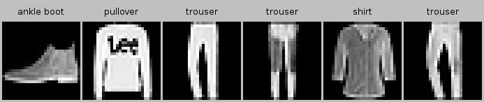
现在训练已经完成,我们的模型已经准备好对图像进行分类预测。给定一系列图像,我们将比较它们的实际标签(文本输出的第一行)和模型预测(文本输出的第二行)。
// Number should be < batchSize for this function to work properly
public BufferedImage predictCh3(UnaryOperator<NDArray> net, ArrayDataset dataset, int number, NDManager manager)
    throws IOException, TranslateException {
    final int SCALE = 4;
    final int WIDTH = 28;
    final int HEIGHT = 28;

    int[] predLabels = new int[number];

    for (Batch batch : dataset.getData(manager)) {
        NDArray X = batch.getData().head();
        int[] yHat = net.apply(X).argMax(1).toType(DataType.INT32, false).toIntArray();
        for (int i = 0; i < number; i++) {
            predLabels[i] = yHat[i];
        }
        break;
    }

    return FashionMnistUtils.showImages(dataset, predLabels, WIDTH, HEIGHT, SCALE, manager);
}

predictCh3(Net::net, validationSet, 6, manager);
3.6.8. 小结
借助 softmax 回归,我们可以训练多分类的模型。
softmax 回归的训练循环与线性回归中的训练循环非常相似:读取数据、定义模型和损失函数,然后使用优化算法训练模型。正如你很快就会发现的那样,大多数常见的深度学习模型都有类似的训练过程。
3.6.9. 练习
在本节中,我们直接实现了基于数学定义softmax运算的
softmax函数。这可能会导致什么问题?提示:尝试计算 \(\exp(50)\) 的大小。本节中的函数
crossEntropy是根据交叉熵损失函数的定义实现的。这个实现可能有什么问题?提示:考虑对数的值域。你可以想到什么解决方案来解决上述两个问题?
返回概率最大的标签总是一个好主意吗?例如,医疗诊断场景下你会这样做吗?
假设我们希望使用softmax回归来基于某些特征预测下一个单词。词汇量大可能会带来哪些问题?